This notebook is an archived snapshot of a 48-bar window and its Al Brooks–style AI analysis.
AI Analysis
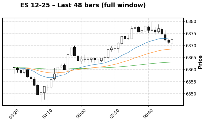
Context: The first ~15–18 bars are a tight, slightly up-sloping trading range around the EMA. Then a bull spike around bars 16–17 leads into a steady bull channel with price and EMA both rising. The last 15–20 bars are a grinding bull channel with small pullbacks and closes mostly above the EMA, but momentum is weakening and the channel is flattening into a possible developing trading range near the highs.
Clear patterns:
Bull spike and channel starting at bar 16 (6866.25 close) through ~bar 35.
Multiple small bull flags / H1-H2 style pullbacks in the channel (e.g., minor dips around bars 18–22, 30–32, 37–42).
Late bull channel with possible “final flag” behavior: higher highs around 35–39, then overlapping bars and small pullbacks (40–47) suggesting loss of momentum and increased risk of a trading-range top or minor reversal.
Probability: Bulls still have the edge because the EMA is rising and pullbacks are shallow, but the buy climax / late-channel context means upside follow-through is less certain and reward is shrinking. Bears are more likely to get a 2–3 leg pullback than an immediate trend reversal, but risk selling too early into a strong bull trend.
With-trend entries / avoids:
Best with-trend buys were earlier: pullback after the spike (around bars 18–22), and subsequent higher low pullbacks within the channel (around bars 30–32, 37–39).
At current bars (mid–high 6870s, 40–47), new longs are late in a mature bull channel and near a possible trading-range top—scalp-only and only on clear bull reversal bars off the EMA.
Avoid initiating fresh shorts until you see a clear bear breakout with follow-through below the recent higher lows (e.g., a strong break and close below the lows of bars 45–47); before that, it’s still “buy the pullback” but with reduced size and modest profit targets.
# RTH-only candlestick chart (example 08:30–15:15 session hours)# Note: adjust the times to your actual RTH / time zone if needed.ifisinstance(df_ohlc.index, pd.DatetimeIndex):# Example: filter between 08:30 and 15:15 (local time) for each day df_rth = df_ohlc.between_time("08:30", "15:15")else: df_rth = df_ohlc.copy() # fallbackiflen(df_rth) ==0:print("No RTH bars found with the given time window; showing full window instead.") df_rth = df_ohlc.copy()ema_overlays_rth = [ mpf.make_addplot(df_rth['EMA20'], width=1), mpf.make_addplot(df_rth['EMA48'], width=1), mpf.make_addplot(df_rth['EMA200'], width=1),]fig, axlist = mpf.plot( df_rth,type='candle', style='classic', addplot=ema_overlays_rth, figsize=(10, 5), title=f"{instrument} – RTH subset (example 08:30–15:15)", ylabel='Price', returnfig=True)plt.show()
# Simple pattern detection: double tops/bottoms and 3-swing wedges## This is intentionally conservative and approximate:# - Finds local swing highs/lows# - Looks for last pair of swing highs within a small price band => DT# - Looks for last pair of swing lows within a small price band => DB# - Looks for last 3 swing highs that are successively higher => wedge up# - Looks for last 3 swing lows that are successively lower => wedge downimport numpy as npdf_sw = df_ohlc.copy()# Identify swing highs/lowsswing_high = []swing_low = []close = df_sw['Close'].valueshigh = df_sw['High'].valueslow = df_sw['Low'].valuesfor i inrange(1, len(df_sw) -1):# simple 3-bar swing definitionif high[i] > high[i-1] and high[i] >= high[i+1]: swing_high.append(i)if low[i] < low[i-1] and low[i] <= low[i+1]: swing_low.append(i)swing_high = np.array(swing_high, dtype=int)swing_low = np.array(swing_low, dtype=int)dt_indices = []db_indices = []wedge_up_indices = []wedge_down_indices = []# Double tops: last 2 swing highs within a bandiflen(swing_high) >=2: i1, i2 = swing_high[-2], swing_high[-1] price1, price2 = high[i1], high[i2]# tolerance as fraction of priceifabs(price2 - price1) <=0.25* df_sw['Close'].iloc[-1]: # adjust tolerance as needed dt_indices = [i1, i2]# Double bottoms: last 2 swing lows within a bandiflen(swing_low) >=2: i1, i2 = swing_low[-2], swing_low[-1] price1, price2 = low[i1], low[i2]ifabs(price2 - price1) <=0.25* df_sw['Close'].iloc[-1]: # adjust tolerance as needed db_indices = [i1, i2]# Wedge up: last 3 swing highs successively higheriflen(swing_high) >=3: i1, i2, i3 = swing_high[-3], swing_high[-2], swing_high[-1]if high[i1] < high[i2] < high[i3]: wedge_up_indices = [i1, i2, i3]# Wedge down: last 3 swing lows successively loweriflen(swing_low) >=3: i1, i2, i3 = swing_low[-3], swing_low[-2], swing_low[-1]if low[i1] > low[i2] > low[i3]: wedge_down_indices = [i1, i2, i3]print("Swing highs:", swing_high)print("Swing lows :", swing_low)print("Double top indices :", dt_indices)print("Double bottom indices:", db_indices)print("Wedge up indices :", wedge_up_indices)print("Wedge down indices :", wedge_down_indices)# Plot with annotations on the full windowfig, axlist = mpf.plot( df_ohlc,type='candle', style='classic', figsize=(10, 5), returnfig=True)ax = axlist[0]x_vals = np.arange(len(df_ohlc))# Annotate DTsfor i in dt_indices: dt_x = x_vals[i] dt_y = high[i] ax.scatter(dt_x, dt_y, s=50, marker='^') ax.text(dt_x, dt_y, 'DT', fontsize=8, va='bottom', ha='center')# Annotate DBsfor i in db_indices: db_x = x_vals[i] db_y = low[i] ax.scatter(db_x, db_y, s=50, marker='v') ax.text(db_x, db_y, 'DB', fontsize=8, va='top', ha='center')# Annotate wedge upfor i in wedge_up_indices: wx = x_vals[i] wy = high[i] ax.scatter(wx, wy, s=40, marker='o') ax.text(wx, wy, 'WU', fontsize=8, va='bottom', ha='center')# Annotate wedge downfor i in wedge_down_indices: wx = x_vals[i] wy = low[i] ax.scatter(wx, wy, s=40, marker='o') ax.text(wx, wy, 'WD', fontsize=8, va='top', ha='center')ax.set_title(f"{instrument} – Simple DT/DB & wedge annotations")plt.tight_layout()plt.show()