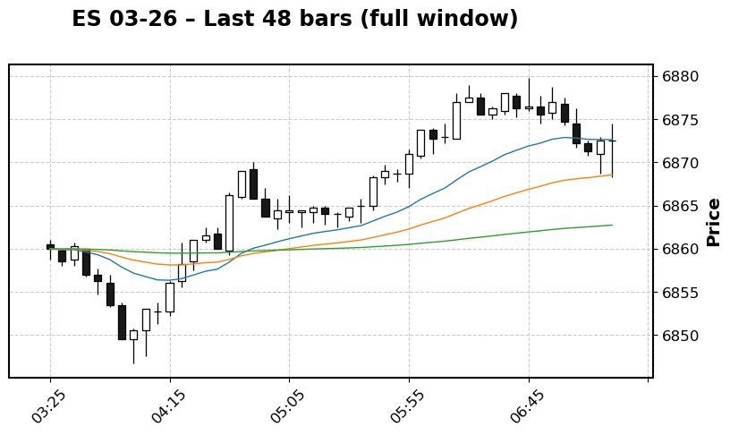
This notebook is an archived snapshot of a 48-bar window and its Al Brooks–style AI analysis.
AI Analysis
Context: The EMA is rising the entire sample and price is mostly above it, so this is a bull trend / bull spike-and-channel that evolved into a tighter bull channel from about bar 27 onward. The early part (0–10) is a flat, slightly down drift around EMA that becomes a clear upside spike around 15–18, then a channel up into the high 6870s.
Clear patterns:
Bull spike at 15–16 followed by a pullback to 18–21 and then a channel up (spike & channel bull trend).
Repeated small bull flags / H2-like setups around 18–21 and again around 25–27.
Latest bars (40–47) form a weak trading-range-like pause / small pullback just above a flattening EMA, potentially a final flag in a mature bull channel.
Probabilities: Bulls still have a slight edge because the EMA is up and price is holding above it, but the channel is aging and momentum is waning; odds of a deeper pullback or transition into a trading range are increasing. This is no longer an early, high-probability bull breakout phase.
Entries / avoid: With-trend buys were best on the pullback near 18–21 and again on the shallow pullback around 36–41. At the current bars (44–47), risk–reward for new longs is mediocre: buying here is late in the channel and vulnerable to a test down toward the EMA or the 6868–6870 area. Avoid fading (shorting) aggressively in the middle of this range; if shorting, it’s better to wait for a clear lower high and strong bear breakout below the EMA rather than guessing tops in this tight structure.
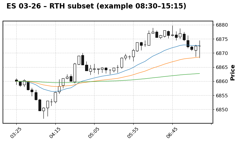
# RTH-only candlestick chart (example 08:30–15:15 session hours)# Note: adjust the times to your actual RTH / time zone if needed.ifisinstance(df_ohlc.index, pd.DatetimeIndex):# Example: filter between 08:30 and 15:15 (local time) for each day df_rth = df_ohlc.between_time("08:30", "15:15")else: df_rth = df_ohlc.copy() # fallbackiflen(df_rth) ==0:print("No RTH bars found with the given time window; showing full window instead.") df_rth = df_ohlc.copy()ema_overlays_rth = [ mpf.make_addplot(df_rth['EMA20'], width=1), mpf.make_addplot(df_rth['EMA48'], width=1), mpf.make_addplot(df_rth['EMA200'], width=1),]fig, axlist = mpf.plot( df_rth,type='candle', style='classic', addplot=ema_overlays_rth, figsize=(10, 5), title=f"{instrument} – RTH subset (example 08:30–15:15)", ylabel='Price', returnfig=True)plt.show()
No RTH bars found with the given time window; showing full window instead.
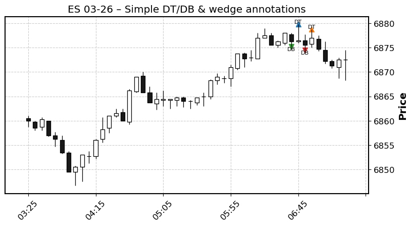
# Simple pattern detection: double tops/bottoms and 3-swing wedges## This is intentionally conservative and approximate:# - Finds local swing highs/lows# - Looks for last pair of swing highs within a small price band => DT# - Looks for last pair of swing lows within a small price band => DB# - Looks for last 3 swing highs that are successively higher => wedge up# - Looks for last 3 swing lows that are successively lower => wedge downimport numpy as npdf_sw = df_ohlc.copy()# Identify swing highs/lowsswing_high = []swing_low = []close = df_sw['Close'].valueshigh = df_sw['High'].valueslow = df_sw['Low'].valuesfor i inrange(1, len(df_sw) -1):# simple 3-bar swing definitionif high[i] > high[i-1] and high[i] >= high[i+1]: swing_high.append(i)if low[i] < low[i-1] and low[i] <= low[i+1]: swing_low.append(i)swing_high = np.array(swing_high, dtype=int)swing_low = np.array(swing_low, dtype=int)dt_indices = []db_indices = []wedge_up_indices = []wedge_down_indices = []# Double tops: last 2 swing highs within a bandiflen(swing_high) >=2: i1, i2 = swing_high[-2], swing_high[-1] price1, price2 = high[i1], high[i2]# tolerance as fraction of priceifabs(price2 - price1) <=0.25* df_sw['Close'].iloc[-1]: # adjust tolerance as needed dt_indices = [i1, i2]# Double bottoms: last 2 swing lows within a bandiflen(swing_low) >=2: i1, i2 = swing_low[-2], swing_low[-1] price1, price2 = low[i1], low[i2]ifabs(price2 - price1) <=0.25* df_sw['Close'].iloc[-1]: # adjust tolerance as needed db_indices = [i1, i2]# Wedge up: last 3 swing highs successively higheriflen(swing_high) >=3: i1, i2, i3 = swing_high[-3], swing_high[-2], swing_high[-1]if high[i1] < high[i2] < high[i3]: wedge_up_indices = [i1, i2, i3]# Wedge down: last 3 swing lows successively loweriflen(swing_low) >=3: i1, i2, i3 = swing_low[-3], swing_low[-2], swing_low[-1]if low[i1] > low[i2] > low[i3]: wedge_down_indices = [i1, i2, i3]print("Swing highs:", swing_high)print("Swing lows :", swing_low)print("Double top indices :", dt_indices)print("Double bottom indices:", db_indices)print("Wedge up indices :", wedge_up_indices)print("Wedge down indices :", wedge_down_indices)# Plot with annotations on the full windowfig, axlist = mpf.plot( df_ohlc,type='candle', style='classic', figsize=(10, 5), returnfig=True)ax = axlist[0]x_vals = np.arange(len(df_ohlc))# Annotate DTsfor i in dt_indices: dt_x = x_vals[i] dt_y = high[i] ax.scatter(dt_x, dt_y, s=50, marker='^') ax.text(dt_x, dt_y, 'DT', fontsize=8, va='bottom', ha='center')# Annotate DBsfor i in db_indices: db_x = x_vals[i] db_y = low[i] ax.scatter(db_x, db_y, s=50, marker='v') ax.text(db_x, db_y, 'DB', fontsize=8, va='top', ha='center')# Annotate wedge upfor i in wedge_up_indices: wx = x_vals[i] wy = high[i] ax.scatter(wx, wy, s=40, marker='o') ax.text(wx, wy, 'WU', fontsize=8, va='bottom', ha='center')# Annotate wedge downfor i in wedge_down_indices: wx = x_vals[i] wy = low[i] ax.scatter(wx, wy, s=40, marker='o') ax.text(wx, wy, 'WD', fontsize=8, va='top', ha='center')ax.set_title(f"{instrument} – Simple DT/DB & wedge annotations")plt.tight_layout()plt.show()
Swing highs: [ 2 13 17 20 22 28 35 38 40 42]
Swing lows : [ 1  7 15 19 21 24 26 30 37 39 41]
Double top indices   : [40, 42]
Double bottom indices: [39, 41]
Wedge up indices     : []
Wedge down indices   : []
C:\Users\markl\AppData\Local\Temp\ipykernel_44724\1182744269.py:114: UserWarning: This figure includes Axes that are not compatible with tight_layout, so results might be incorrect.
  plt.tight_layout()